I presented Moody and Saffell's Learning to Trade via Direct Reinforcement (IEEE TNN, 2001) in my Investments class, and reproduced their results along the way. These are short notes on the method.
Moody did some of the earliest work on avoiding the need of forecasting models in financial markets and directly learn an optimal strategy which they call direct reinforcement.
# Trading System
Let be the price of the traded asset at time , and its price change over the last period. At each step the trader holds a position : long, neutral or short. The position is a function of the trader's parameters, its previous position and everything it has seen so far,where is the information set. Basically, a trader is a single recurrent unit that looks at its last position and the last price changes,
We can also write , where so , and . Note that during training the sign is smoothed to a so that is differentiable. With position size and transaction cost , the trading return over period is
which is just the profit from the position held over the period, minus the cost of changing positions.
Instead of forecasting prices or learning a value function, Recurrent Reinforcement Learning (RRL) adjusts by gradient ascent directly on a trading performance measure. Moody and Saffell repurposed the sharpe ratio to enable on-line optimization. The differential Sharpe ratio is the first-order effect of the latest return on an exponential moving Sharpe ratio. This was their objective for measuring risk adjusted returns. To measure risk, they formulated the differential downside deviation. It is analogous to the sterling ratio (just because it is very hard to minimize drawdowns). The paper also compares this direct reinforcement approach with Q-learning on monthly S&P 500 / T-bill allocation. In my notes, I will just show the differential Sharpe Ratio, since the differential downside deviation follows the same derivation.
# Differential Sharpe Ratio
We want to maximize the Sharpe ratio over periods,
But, the Sharpe ratio is a statistic of the whole history, and we want to update after every trade. To solve this, we can keep exponential moving averages of and ,
and expand the moving Sharpe ratio to first order in . The first-order term is the differential Sharpe ratio:
is the marginal effect of the recent return on the Sharpe ratio.
# The algorithm
Since depends on , the gradient has to be carried forward in time, as in real-time recurrent learning.
Algorithm 1: Recurrent Reinforcement Learning (RRL)
Require: learning rate , EMA rate , transaction cost
# Results
Moody and Saffell performed a bunch of experiments. First, the generated synthetic data to see RRL algorithms learns to make optimal trading strategies. The trader in this experiment has 10 weights. Over 100 random markets it had a positive Sharpe ratio every time, and it learned on its own to trade less as costs went up, from about 6% of periods at 0.2% cost to about 3% at 1%.
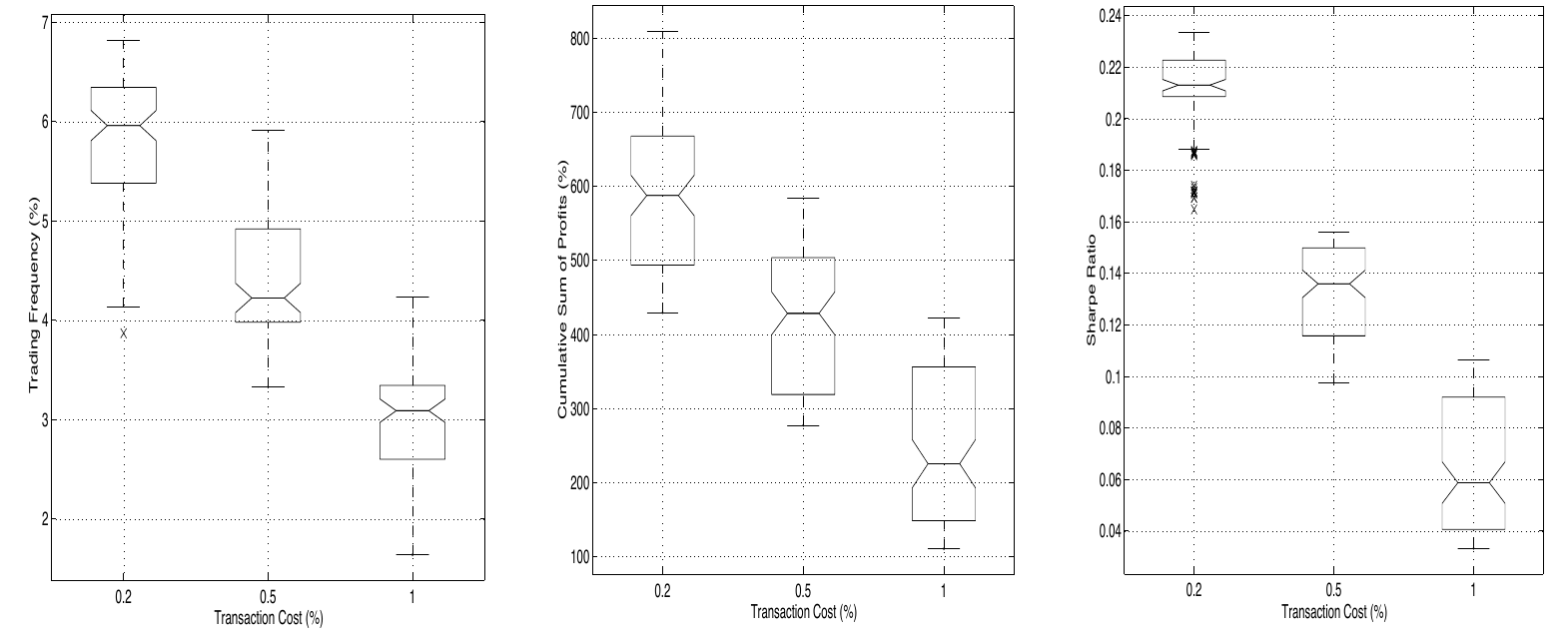
Figure 1: Trading frequency, cumulative profit and Sharpe ratio against transaction cost, over 100 trials on artificial data. From Moody and Saffell (2001), Fig. 5, © IEEE.
In the second experiment they trained and evaluated the RRL algorithm on actual US Dollar/British Pound Foreign Exchange Rates from 1996 using the differential downside objective (you just change line 7, in algorithm 1). It performed well, and also interestingly learned to reduce trading frequency with rising transaction costs. The trading system achieved an annualized Sharpe ratio of 2.3 and annualized 15% return over approx 6 months out-of-sample test period. On average, the system made a transaction per 5 hours. However, in my implementations, I tried this with USD/GBP FX data from 2010 and go very poor results. I am currently investigating this as part of my final project for the Investments class. I suspect an obvious expressivity issue that hinders representations because of the the shallow network.
The third experiment was conducted on the S&P 500 against Treasury bills, 1970 to 1994, the RRL trader is also a single unit. Because one trader's result depends on its random initial weights, the paper trains 30 of them independently and trades their combined position. The Q-learning baseline (30 hidden units) is evaluated the same way. The RRL ensemble ended at about 59 times its starting wealth, against 34 times for the Q-learning ensemble and 13.5 times for buy and hold, with annualized Sharpe ratios of 0.83, 0.63 and 0.34. Most of the edge came from moving into T-bills at the right times including the 1974 oil shock, the early-1980s rate spike and the 1987 crash.
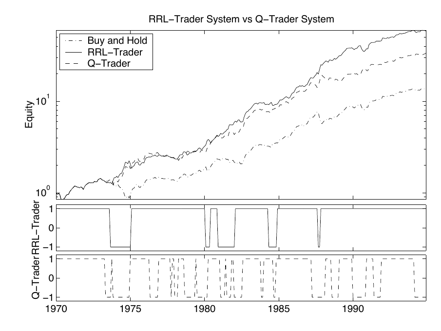
Figure 2: Equity of the RRL and Q-trader committees and buy and hold, 1970 to 1994, with each committee's position below. From Moody and Saffell (2001), Fig. 9, © IEEE.
# References
- J. Moody and M. Saffell, Learning to Trade via Direct Reinforcement, IEEE Transactions on Neural Networks 12(4), 2001;
- J. Moody, L. Wu, Y. Liao and M. Saffell, Performance Functions and Reinforcement Learning for Trading Systems and Portfolios, Journal of Forecasting 17, 1998.