#1. Motivation
Recent work trains language models by self-play on zero-sum games. SPIRAL (Liu et al., 2026) have used poker and other games to improve reasoning. 1 Some of this work relies on training reaching an equilibrium. Self-RedTeam (Liu et al., 2025) work pits an attacker against a defender to improve safety, and argues that the defender is safe at an equilibrium. 2 In a two-player zero-sum game, a Nash equilibrium is a pair of strategies where neither player can gain by changing theirs. An equilibrium strategy earns at least the game's value against any opponent. A strategy's exploitability is how much an opponent who knows the strategy and plays the best counter to it (a best response) wins on average. Exploitability is zero at an equilibrium. Thus, a model with positive exploitability can be exploited. There exists some opponent who wins more against it than against an equilibrium.
#1.1 Contributions
We study three small instruct models from two families, Qwen2.5 (0.5B and 1.5B) and SmolLM2-1.7B, fine-tuned with LoRA. The two families start have opposite biases where Qwen bets almost always, and SmolLM2 mostly checks in Kuhn Poker.
- We read an LLM's exact policy at every decision point of Kuhn poker and track its exploitability exactly throughout self-play training. (Section 3)
- In both model families, we find that at strong KL, a 12-parameter table anchored to the base model's action probabilities predicts where the LLM plateaus. (Section 5.2)
- In the Qwen family, we find that at weak KL, the model never learns to condition on its private card, while a table and SmolLM2 trained with the same recipe do. We test one candidate mechanism and leave the cause open. (Section 5.4)
- Finally, we show that win rate and payoff against fixed opponents rank these exploitable policies inconsistently across models, and sometimes backwards. (Section 5.5)
#2. Exploitability in Small Games
#2.1 Kuhn poker
Kuhn poker is poker reduced to three cards (J, Q, K), one card per player, an ante of 1 chip, and one betting round. 4 Basically, player 1 checks or bets; when facing a bet, a player calls or folds; after a check, player 2 may check or bet. A player's information set (decision point) is their own card and the betting so far. Kuhn poker has 12 information sets. Its equilibria are known in closed form.
For a policy that plays both players, exploitability is:
#2.2 Rock-Paper-Scissors
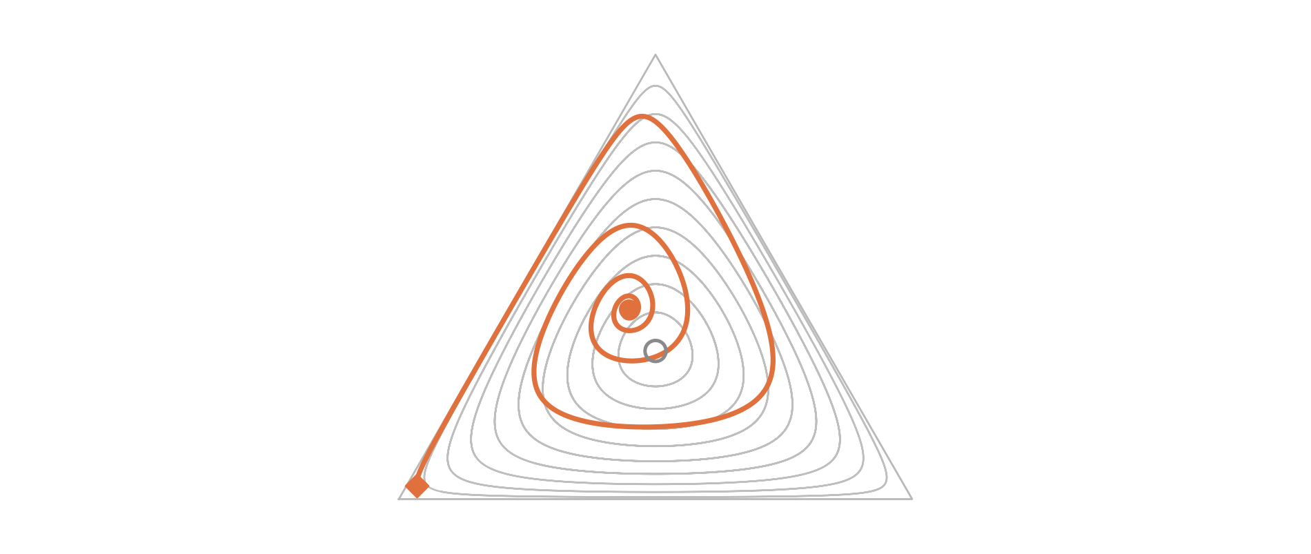
We demonstrate the learning dynamics on rock-paper-scissors. Consider every strategy as a point in a triangle and the equilibrium ( each) is the center. Below, one policy plays itself and moves toward whatever beats its current mix. It starts at a base model that plays rock 95% of the time, as Qwen2.5-0.5B does before training.
Training settles at the ring. It is stable, but still exploitable.
Figure 1 (interactive): This is an illustration, it is not an experiment we ran. Rock-paper-scissors self-play with a KL penalty. Without KL (1), training circles the equilibrium. KL to the biased base model (2, 3) stops the circling at a stable, exploitable point. A uniform anchor (4) lands on the equilibrium only because this game's equilibrium is uniform. Moving the anchor and averaging (5) reaches equilibrium. Self-play reward is 0 throughout, since a policy always breaks even against itself.
From this figure, we observe the following and test each in Kuhn poker with LLMs:
- The anchor stabilizes training.
- At a fixed anchor and strength , the resting policy at each decision point is . So, a biased anchor gives a biased and exploitable resting point.
- The training signal is symmetric, so a policy's reward against itself says nothing about how exploitable it is.
#3. Method
#3.1 The Model as a Policy
The game state is rendered as text where the model answers with one action word. Here is player 2, holding a K, after player 1 checked:You are playing Kuhn poker as Player 2.
Rules: the deck has three cards, J, Q and K (K is highest). Each player antes 1 chip and is dealt one card.
Player 1 acts first and can check or bet 1 chip. If Player 1 checks, Player 2 can check (go to showdown) or bet 1 chip.
A player facing a bet can call (match the bet, then showdown) or fold (give up the pot). At showdown the higher card wins the pot.
Your card: K
Betting so far: Player 1 checked.
Reply with exactly one word: check or bet.
Formally, let be the prompt for information set , and let action word tokenize as . We score each legal action word by the summed log-probability of its tokens after the assistant header:
The policy is a softmax over the legal actions only:
We pass the exact distribution to OpenSpiel 5 to compute exploitability exactly, with no sampling noise. Read more on Counterfactual Regret Minimization in my Notes.
#3.1 Tabular Policies
To separate the training algorithm from the LLM, every experiment has a tabular counterpart trained with an identical loop. It has one free logit per information set, the same loss, KL, advantages and batch size. The table's learning rate is not comparable to the LLM's. For the table, it moves each action logit directly. For the LLM it updates the LoRA weights, and how far that shifts the policy depends on the network. A step of one is therefore not a step of the other, so we can only compare policies' late-training behavior.
If the LLM's plateau is the regularized point of its base model, a table given only the base model's 12 action probabilities, as both its starting policy and its anchor, should land in the same place. We read those probabilities from step 0 of each LLM run (the exact anchor the LLM was trained against) and train the table for 3000 steps. Before looking at the results, we fixed a match criterion where at all 12 decision points, the table's seed mean must lie within the LLM's seed range ± 0.05, and its exploitability within ± 0.02. We judge the table both at its last iterate and averaged over the second half of training (reach-weighted, as in CFR), and report both.
To test whether coupling between information sets can explain the LLM's failure to use its card, we build a table whose cards share part of their logits:
For same-signed gradients, the cosine between two cards' parameter gradients is then , so gives 0.99, the value we measure in the LLM. The coupled table has the same start and anchor as the free table.
#4. Experimental Setup
Models. We use Qwen2.5-0.5B-Instruct, Qwen2.5-1.5B-Instruct and SmolLM2-1.7B-Instruct each with a LoRA adapter (rank 16, attention projections). All three models are card-blind before training (identical probabilities with J, Q and K) but they are biased in different directions. Qwen2.5-0.5B bets about 0.96 of the time everywhere; Qwen2.5-1.5B calls about 0.9 of the time and opens with a J 0.33 of the time. SmolLM2 checks about 0.86 of the time when opening and calls 0.5-0.64 of the time.
Training algorithm. We follow the training choices of Liu et al in SPIRAL 1 and Liu et al in Self-RedTeam 2. We play one model in both seats and train it by policy gradient on game outcomes, with 512 self-play hands per step. Each batch receives a single update, so the GRPO objective 6 reduces to REINFORCE. We normalize advantages separately for each seat, by the batch mean and standard deviation. And, we compute the KL penalty to the base model exactly over the legal actions rather than estimated from samples. Our main runs use KL 0.25 and learning rate 5e-6.
Runs. We run 1000 steps for LLMs and 3000 steps for tables, with 3 seeds per configuration. We log exploitability, the probability at each information set, and payoff and win rate against a uniform random player and against OpenSpiel's CFR equilibrium policy. 7
Verification. We cross-check exploitability against a brute-force best response over all 64 pure strategies per player. The policy readout was broken on purpose three ways (padding, an off-by-one logit slice, scoring only a word's first token) to confirm the tests catch each one. We wrote 65 tests.
#5. Results
Self-play makes every model less exploitable but stops short of equilibrium (5.1). The base model predicts where it stops (5.2), and the anchor is the cause (5.3). At weak KL, a second limit appears that the training algorithm alone does not explain (5.4). The metrics used in LLM self-play papers detect none of this (5.5), and the standard fixes help the table far more than the LLM (5.6).
#5.1 Self-play improves every model, but each one plateaus short of equilibrium
At KL 0.25, every model ends less exploitable than it started (Figure 2). Qwen2.5-0.5B goes from 0.53 to about 0.19, Qwen2.5-1.5B from 0.35 to about 0.20, and SmolLM2 from 0.42 to about 0.09. None of them reaches equilibrium. Qwen2.5-0.5B ends at 0.197, 0.185 and 0.202 on three seeds, and a 3000-step run stays between 0.192 and 0.200 in every 500-step window. Observe that exploitability stops falling and holds at a level above zero, so more training does not bring the model closer to equilibrium, thus a plateau.
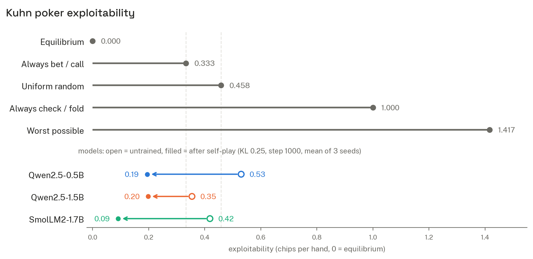
Figure 2: Self-play makes every model less exploitable than a policy that ignores its card (0.333).
The remaining mistakes follow each base model's bias (Table 1). The Qwen models start out betting almost always, and they still bet and call too often. SmolLM2 starts out checking, and it still bets too rarely.
| Model | Decision point | Trained policy | Equilibrium |
|---|---|---|---|
| Qwen2.5-0.5B | Open (bet) with J | 0.80 | at most 1/3 |
| Qwen2.5-0.5B | Open (bet) with Q | 0.93 | never |
| Qwen2.5-1.5B | Call a bet with J | 0.56 | never (always loses) |
| SmolLM2-1.7B | Bet with K after a check | 0.29 | always |
Table 1: The largest remaining mistakes at KL 0.25 point in the direction of each base model's bias. Values are the probability of the action.
#5.2 The base model's 12 action probabilities predict the plateau
We start a table at the base model's 12 action probabilities, anchor it to them, and train it with the same algorithm as the LLM (Section 3). The table reaches the LLM's plateau height for all three models (Figure 3).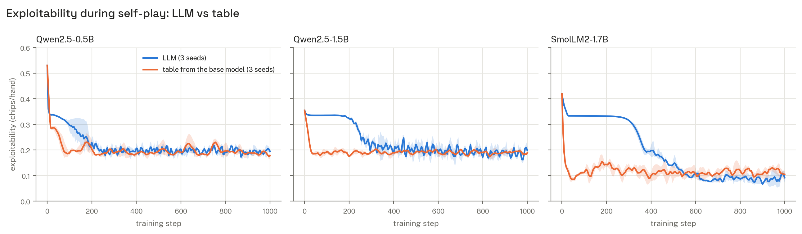
Figure 3: At KL 0.25, the table trained from the base model's probabilities (orange) settles at the LLM's plateau height (blue) for all three models. The table's learning rate has no LLM equivalent, so compare plateau heights, not how fast each gets there. Line = seed mean, band = range over 3 seeds.
The table also matches the LLM decision point by decision point (Figure 4). The prediction matches for SmolLM2 and Qwen2.5-1.5B, and partly matches for Qwen2.5-0.5B by the criterion we set in Section 3. (Table 2). Qwen2.5-0.5B's two misses are both player 2 betting after a check, with a Q (off by 0.06–0.10) and with a K (off by 0.01).
| Model | Decision points matched (last iterate / averaged) | Exploitability: table vs LLM | Verdict |
|---|---|---|---|
| SmolLM2-1.7B | 12/12 / 12/12 | 0.06–0.11 vs 0.09 | match |
| Qwen2.5-1.5B | 10/12 / 12/12 | 0.18–0.19 vs 0.20 | match (averaged table) |
| Qwen2.5-0.5B | 10/12 / 10/12 | 0.19–0.20 vs 0.19 | partial |
Table 2: The run is setup according to Section 4. Prediction from the base model at KL 0.25.
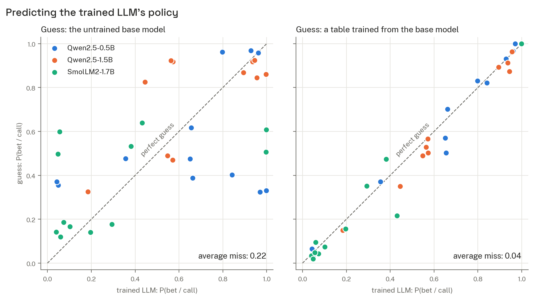
Figure 4: Each dot is one decision point for one model. Dots on the dashed diagonal mean the guess equals what the trained LLM actually does. The untrained base model alone is a poor guess (left, average miss 0.22). The table trained from it is a good one (right, average miss 0.04). KL 0.25, mean of 3 seeds.
For these models, where KL 0.25 self-play plateaus can be computed from the untrained model's action probabilities in a few CPU minutes, without training the LLM.
#5.3 Changing the anchor moves the plateau, but changing the KL strength does not
Table 3 tests whether changing the KL strength removes the plateau by changing the anchor to a uniform distribution using Qwen2.5-0.5B.
| KL | Anchor | Exploitability (late mean) | Behavior |
|---|---|---|---|
| 0.04 | base | 0.333 | collapses to card-blind always bet/call (Section 5.4) |
| 0.1 | base | 0.17–0.19 | unstable: J opening bet swings between 0.05 and 0.95 |
| 0.25 | base | 0.195–0.197 | plateau |
| 1.0 | base | 0.263–0.268 | stays near the base model (J opening bet 0.97) |
| 0.25 | uniform | 0.093–0.095 | J opening bet 0.23, inside the equilibrium range |
Table 3: KL strength and anchor, Qwen2.5-0.5B, 3 seeds per row, 1000 steps, learning rate 5e-6; late mean = steps 500–1000.
We find that none of the KL strengths works with the base model as the anchor. The weak penalty collapses play, and a strong penalty keeps the policy closer to the base model's bias. Replacing the anchor with a uniform distribution at the same strength halves exploitability. This is a diagnostic, not a fix: a uniform anchor exists only because the action set is small and known. The remaining 0.09 also appears in a table trained with the same uniform anchor, so it comes from the training algorithm, not the LLM.
#5.4 At weak KL, Qwen never learns to use its card, although the same algorithm on a table does
Facing a bet, a player that uses its card should call with a K and fold with a J. Figure 5 tracks this gap at KL 0.04. A table trained with the same algorithm, from the same start, learns it within about 20 steps. SmolLM2 learns it by step 750. Neither Qwen model ever does: both call every bet with every card, including a J, which always loses. Qwen2.5-0.5B ends at exploitability 0.333 on all three seeds, the value of always betting and calling, and SPIRAL's settings give the same result.
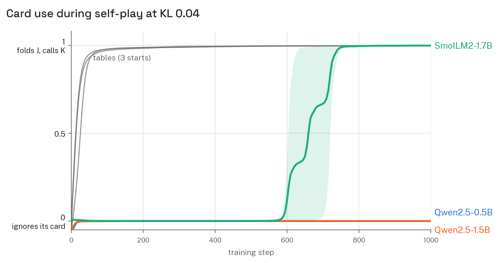
Figure 5: At KL 0.04, the tables and SmolLM2 learn to fold a J and call a K; both Qwen models play every card the same way for the whole run. The y-axis is P(call with K) − P(call with J) when facing a bet: 1 means folding a J and calling a K, as at equilibrium; 0 means ignoring the card. Line = mean of 3 seeds, band = range.
We believe that the limit is not the model's capacity. With supervised training and the same adapter, Qwen2.5-0.5B learns to fold a J and call a K within 20 steps. Why self-play does not find this is still open. Qwen's gradients for the three cards are nearly parallel (cosine 0.99), so every update moves them together, and a table whose updates are coupled this strongly also freezes at most decision points. But SmolLM2's gradients are just as parallel, and it escapes.
#5.5 Payoff metrics do not track exploitability
LLM self-play papers report win rate against other models or payoff against the equilibrium. Figure 6 compares each model's KL 0.25 run with its more exploitable KL 0.04 run on the two closest metrics we can compute.
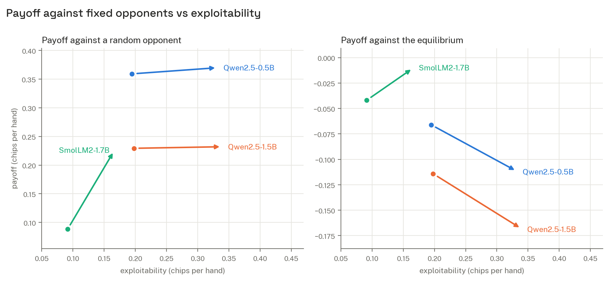
Figure 6: Each arrow goes from a model's KL 0.25 run (dot) to its more exploitable KL 0.04 run; a metric that tracked exploitability would fall along every arrow. Moving to the more exploitable run never lowers payoff against a random opponent (left). Payoff against the equilibrium falls for Qwen but rises for SmolLM2 (right).
We find that:
A weak opponent rewards policies that exploit it, not policies that are hard to exploit. Therefore, payoff against a random opponent never falls, and for SmolLM2 it rises from 0.09 to 0.22.
Payoff against the equilibrium ranks the Qwen runs correctly but SmolLM2's backwards.
Self-play reward cannot help either since with one shared policy, the two seats' rewards mirror each other.
#5.6 A moving anchor with averaging helps the table far more than the LLM
From figure 1, we get the idea to average the policy over training, and move the anchor to the current policy every steps, as in magnetic mirror descent and R-NaD. 3 Averaging alone does nothing for the LLM (0.195 becomes 0.19), because its policy is not oscillating; it sits at a fixed point. Moving the anchor and averaging takes the table to 0.012–0.018, but the LLM only to 0.054–0.150, depending on the seed (Table 4). Once the LLM is anchored to its own policy, it turns near-deterministic, and in 3000 steps it visits too few strategies for their average to converge.
| Run (Kuhn, KL 0.25) | Last iterate (2nd-half mean) | Averaged policy |
|---|---|---|
| Table, fixed anchor | 0.11–0.12 | 0.076–0.078 |
| LLM (Qwen2.5-0.5B), fixed anchor | 0.195–0.197 | 0.19 |
| Table, moving anchor N = 50 | 0.079–0.084 | 0.012–0.018 |
| Table, moving anchor N = 100 | 0.065–0.077 | 0.013–0.018 |
| LLM, moving anchor N = 100 | 0.164–0.167 | 0.118–0.147 |
| LLM, moving anchor N = 200 | 0.131–0.266 | 0.054–0.150 |
Table 4: Fixed-anchor averages use the second half of training (1000 steps); moving-anchor runs are 3000 steps, averaged over all steps. 3 seeds each.
#6. Discussion
KL-regularized self-play inherits more from pretraining than from the game. This makes stability and win rate poor evidence of equilibrium, since a self-play model can be both stable and strong against fixed opponents while staying exploitable in the direction of its base model's bias. With the base model as a fixed anchor there is no good KL strength, so LLM self-play likely needs an anchor that stays mixed, such as an average of past policies, or a population of opponents. We leave testing these, and explaining why SmolLM2 escapes the card-blind freeze while Qwen does not, to future work.
#6.1 Limitations
We used small models (0.5B to 1.7B parameters), trained with LoRA, and pick one-word actions from a single prompt format without reasoning, in a game with only 12 decision points; SPIRAL, by contrast, fully fine-tunes Qwen3-4B with reasoning. The plateau and metric results hold across two model families, but we do not claim they extend to larger models or to reasoning. The KL coefficient of 0.25 is our choice, made because the papers' defaults collapse Qwen2.5-0.5B, so we claim only that SPIRAL's settings collapse this model, not that SPIRAL's own models are card-blind. Finally, each configuration has only three seeds which is not enough to draw stronger conclusions about the stability of the results.
#7. Reproducibility
Compute. All runs used two NVIDIA RTX A5000 GPUs (24 GB each). Each LLM run trains a LoRA adapter (rank 16, on the attention projections) for 1000 steps of 512 self-play hands, so about half a million hands per run, and computes exact exploitability every 5 steps. One seed takes about 11 minutes for Qwen2.5-0.5B, 43 minutes for Qwen2.5-1.5B and 54 minutes for SmolLM2-1.7B. The two larger models need gradient checkpointing to fit in 24 GB. The main results (three models, KL 0.25 and 0.04, three seeds each) take about 11 GPU-hours, and every experiment in this post takes about 20. The tables run on a CPU in a few minutes each.Everything I used, including code, configs, logged metrics and figures, is at github.com/divinrkz/exploitable-selfplay.
Each experiment is a config file plus a seed, and each run saves its full config, the git commit and the package versions next to its metrics. REPRODUCE.md lists every config with its seeds and runtime, and every model is pinned to a Hugging Face commit.
uv venv --python 3.13 .venv
uv pip install --python .venv/bin/python --index-strategy unsafe-best-match -r requirements-lock.txt
uv pip install --python .venv/bin/python -e . --no-deps
.venv/bin/python -m pytest -q

# one LLM self-play run (3 seeds, GPU)
PYTHONPATH=src PYTHON=.venv/bin/python scripts/queue_runs.sh configs/run3_kuhn_selfplay.yaml

# the base-model prediction (CPU)
PYTHONPATH=src PYTHON=.venv/bin/python scripts/queue_runs.sh configs/tabular_run3_kuhn_selfplay_basestart_*.yaml
PYTHONPATH=src .venv/bin/python scripts/e1_prediction.py
PYTHONPATH=src .venv/bin/python scripts/coupled_check.py
#8. On Using AI
I used Claude throughout. For code writing, and fast iteration of cheap experiments. This write-up, however, is largely my interpretation of the experimental results.#9. References
- [1]Liu, Bo, Simon Yu, Zichen Liu, Leon Guertler, Penghui Qi, Daniel Balcells, Mickel Liu et al. "Spiral: Self-play on zero-sum games incentivizes reasoning via multi-agent multi-turn reinforcement learning." In International Conference on Learning Representations, vol. 2026, pp. 35407-35434. 2026.
- [2]Liu, Mickel, et al. "Chasing Moving Targets with Online Self-Play Reinforcement Learning for Safer Language Models." arXiv preprint arXiv:2506.07468 (2025).
- [3]Sokota, Samuel, et al. "A Unified Approach to Reinforcement Learning, Quantal Response Equilibria, and Two-Player Zero-Sum Games." arXiv preprint arXiv:2206.05825 (2022).
- [4]
- [5]Lanctot, Marc, et al. "OpenSpiel: A Framework for Reinforcement Learning in Games." arXiv preprint arXiv:1908.09453 (2019). github.com/google-deepmind/open_spiel
- [6]Shao, Zhihong, et al. "DeepSeekMath: Pushing the Limits of Mathematical Reasoning in Open Language Models." arXiv preprint arXiv:2402.03300 (2024).
- [7]Neller, Todd W., and Marc Lanctot. "An Introduction to Counterfactual Regret Minimization." (2013). modelai.gettysburg.edu/2013/cfr